The next generation of quantum computers will read and write idealized quantum oscillators called qubits. These idealized qubits do not decay, are perfectly isolated from their environment, have an unlimited coherence lifetime, and can selectively entangle with any number of other oscillating quantum qubits. Of course, there are no such qubit ideals and there are all kinds of practical limits to qubits not unlike the practical limits of 0's and 1's in the early days of semiconductor logic bits.
In fact, a real qubit decays and that decay limits the qubits. A real qubit is never perfectly isolated from thermal and phase noise environment and also has a limited phase coherence lifetime on the order of 10 microseconds. There are therefore many hurdles to overcome before any practical qubits of quantum computing become a reality. Much like the early days of the practical 0 and 1 bits of semiconductor logic, Science has a long ways to go in order to realize a useful practical qubit that includes not only 0 and 1, but also quantum phase, theta.
The superconducting Josephson junction is a fundamental quantum oscillator that involves electron (Cooper) pairs tunneling through an insulator layer between two superconductors at very low temperature. Instead of the electrons and holes that determine semiconductor 0 and 1 bits, a Cooper pair is inherently a qubit. For a current of 40 nA, about 1e9 electron pairs result and from a 13 microV, a frequency of 6.6 GHz at 0.015 K. The Cooper pair current results from the specific geometry and materials of the junction as well as the applied voltage but the frequency is always just proportional to the applied voltage. In fact, this junction is a quantum oscillator at that frequency where each excited state includes one additional Cooper pair of electrons at a slightly lower frequency due to anharmonicity.
The basic qubit of a quantum computer incorporates not only the 0 and 1 of a classical bit, but also a quantum oscillation between 0 and 1 of the Cooper pair across a junction. A very common qubit is a particular Josephson junction called a transmon that incorporates a shunt capacitor to make the quantum oscillator more stable. The transmon that oscillates at around 6.6 GHz and so its qubits undergo this same quantum oscillation.
Another common qubit is the squid, which involves a loop with two Josephson junction. In any case, a qubit is the excitation of just one Cooper pair, 0 -> 1, across a junction at about 200 MHz lower frequency due to anharmonicity. The quantum anharmonicity also means that the 1 -> 2 transition is 200 MHz less that then 0 -> 1 transition. In fact, useable qubits need to have such isolated transitions and so the anharmonicity is what makes the transmon and the squid useful qubits as the figure shows.
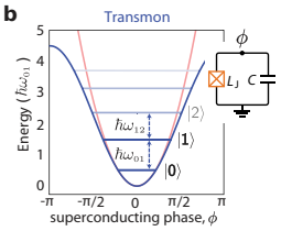
However, there is an additional splitting of each level due to the phase or direction of the electron pair across the junction and that splitting reflects the spin or rotation of the qubit as the figure below shows. Much like electron spin emerges from the complementary rotations of electron charge loop oscillation, the complementary rotations of superconducting loop oscillations in the transmon and squid are then a kind of qubit spin.
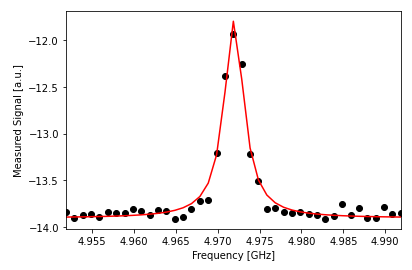
The charge dispersion of the even(+) and odd(-) states depends on many different factors including biasing the gate ng. Gate bias increases charge dispersion up to 60 MHz as the figure shows.
There are literally dozens of other qubit schemes based on Josephson junctions because there are all kinds of practical considerations for reading, writing, and error checking qubits and, of course, adjusting their couplings. For example, it is desirable to have qubit lifetime long enough to allow for useful computation, but short enough to also be quickly reset. So superposition states result from rotating quantum phase by pi/2 or 90d.
The Google Sycamore chip incorporates 27 squid qubit pairs with 88 transmon couplers in a 6x9 zig-zag grid. There is a stability associated with such complementary qubits that is not unlike the bond between two hydrogen atoms. For example, there are many undesirable couplings among qubits simply due to their proximities. Coupling adjacent qubits with complementary spins forms the basis of a swap gate.
The qubit lifetime, T1, is therefore usually about 10 microsec, which is long enough for reading and still short enough for resetting, which all involve 10 nsec switches. The dephasing time, T2, is due to the entanglement among other qubit states that is necessary for effective computation. This dephasing time is important for quantum entanglement outcomes and is therefore limited by T1. However, it is then difficult to differentiate dephasing from pure decay.
Arrays of coupled qubits then become the molecules of the quantum computer and excitations of those molecules are the qubits. It is the evolution of those qubit excitations from an initial to a final state that is the nature of quantum computation. Eventually, the excitation decays completely into incoherent heat and the whole key is to get a useful result before the inevitable decay to incoherence.
The quantum Fourier transform is perhaps the most fundamental quantum computation that shows quantum supremacy over the discrete Fourier transform of a classical digital computer. Although both quantum and classical FT's decompose a bit sequence into a bit spectrum, the quantum time needed is drastically less than the classical time. While the classical time needed is exponential, the quantum time needed is polynomial.
Below are three qubit sequences along with their FT qubit spectra for a qubit sequence at the Nyquist limit, a sinc pulse, and at the low frequency limit. Unlike a digital FT that evolves in exponential time, a quantum FT evolves from a series of operations in polynomial time to factor odd bit sequences by that evolution. Of course, the larger the number, the greater the number of operations needed to factor the number. Currently, 15 is the largest number that quantum computers have factored because of the current limits of coherence and error.


